Chapter 2 Introduction
The motivation for creating the bifrost package at Institute of Marine Research (IMR) is to make the capelin assessment more available and reproducible. There has been a tendency that a single person sits on all the knowledge of how to do the assessment and the necessary estimation of parameters, and when this person is no longer available, those left behind are stranded. So we hope that the bifrost R-package can help in terms of availability, transparency and reproducibilility.
Another issue with how things used to be done, is that different steps in the assessment used different software. You had one program to estimate parameters in the maturing model, for instance, and another to run Monte Carlo simulations based on these estimates. Here we want a unified software package that allows the user do it all within the same framework.
A third element of this project is to move away from having to deal with, say 20 different excel sheets, to load the necessary data for the assessment.
Within the procject, multiple research papers has been published.
This user-guide will explain how to use the package and what the key features are. The book is divided into chapters. Chapter 3 explains how the input data should be structured and Chapter 4 presents how to estimate the maturity model for capelin, while Chapter 5 explains how to run the Monte Carlo simulations. The Chapter 6 explains how the consumption model works.
The following is just kept as example code
par(mar = c(4, 4, .1, .1))
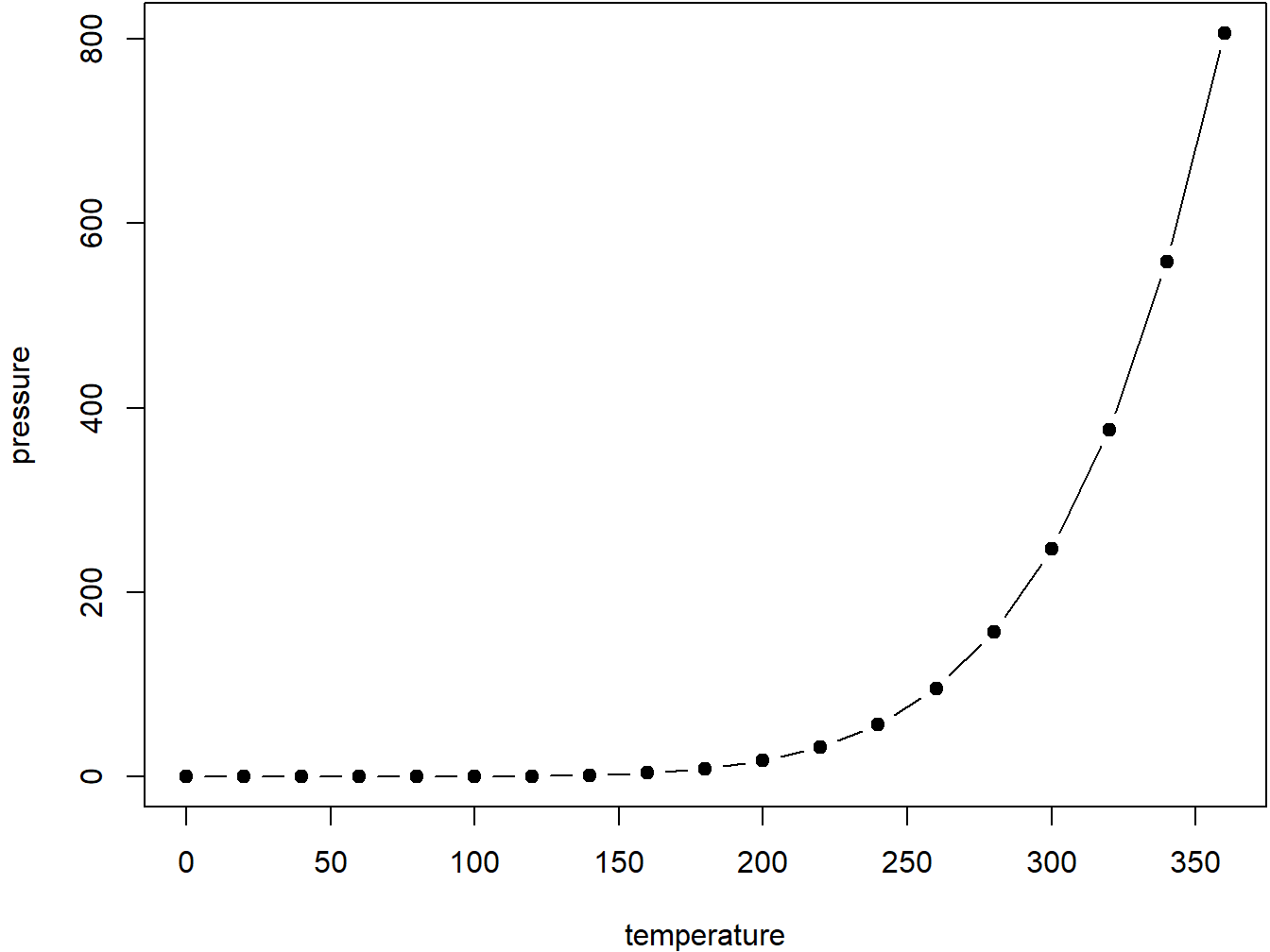
plot(pressure, type = 'b', pch = 19)
Figure 2.1: Here is a nice figure!
Reference a figure by its code chunk label with the fig: prefix, e.g., see Figure 2.1. Similarly, you can reference tables generated from knitr::kable(), e.g., see Table 2.1.
knitr::kable(
  head(iris, 20), caption = 'Here is a nice table!',
  booktabs = TRUE
)| Sepal.Length | Sepal.Width | Petal.Length | Petal.Width | Species |
|---|---|---|---|---|
| 5.1 | 3.5 | 1.4 | 0.2 | setosa |
| 4.9 | 3.0 | 1.4 | 0.2 | setosa |
| 4.7 | 3.2 | 1.3 | 0.2 | setosa |
| 4.6 | 3.1 | 1.5 | 0.2 | setosa |
| 5.0 | 3.6 | 1.4 | 0.2 | setosa |
| 5.4 | 3.9 | 1.7 | 0.4 | setosa |
| 4.6 | 3.4 | 1.4 | 0.3 | setosa |
| 5.0 | 3.4 | 1.5 | 0.2 | setosa |
| 4.4 | 2.9 | 1.4 | 0.2 | setosa |
| 4.9 | 3.1 | 1.5 | 0.1 | setosa |
| 5.4 | 3.7 | 1.5 | 0.2 | setosa |
| 4.8 | 3.4 | 1.6 | 0.2 | setosa |
| 4.8 | 3.0 | 1.4 | 0.1 | setosa |
| 4.3 | 3.0 | 1.1 | 0.1 | setosa |
| 5.8 | 4.0 | 1.2 | 0.2 | setosa |
| 5.7 | 4.4 | 1.5 | 0.4 | setosa |
| 5.4 | 3.9 | 1.3 | 0.4 | setosa |
| 5.1 | 3.5 | 1.4 | 0.3 | setosa |
| 5.7 | 3.8 | 1.7 | 0.3 | setosa |
| 5.1 | 3.8 | 1.5 | 0.3 | setosa |
You can write citations, too. For example, we are using the bookdown package (Xie 2021) in this sample book, which was built on top of R Markdown and knitr (Xie 2015).